
Control loops from on/off to PID: the bases, the four types, and what changes when a PLC runs them
A jacketed vessel has held 37 °C for years. After a valve replacement the temperature starts to swing: 36.2, 37.9, 36.4, 37.7 °C, every four minutes. Someone raises the controller gain “to make it react faster”, and the swing gets wider. Someone else lowers it, and the vessel now settles at 36.6 °C and never reaches its setpoint. Both did what the controller seemed to be asking for. Neither knew which kind of controller was in the loop, or what kind of process it was driving.
None of this is advanced control theory. It is the ground every automation, maintenance and validation engineer on a site should stand on, because every temperature, level, pressure, flow and speed that matters to the product is held by a loop of this kind. This article walks through it: what a loop is made of, how its quality is judged, the four types of controller you will meet, and what changes when the controller is a few lines of PLC code instead of a box on a panel.
Open loop, closed loop, and the two jobs of a loop
In open loop, the command is set without looking at the result: heat at 30 % of full power and hope the oven ends up where you want. It is simple and it cannot become unstable, but it is blind. If the door opens, the load changes or the mains voltage drops, nothing reacts, because nothing measures.
In closed loop, the result is measured, compared with what is wanted, and the command is corrected from the difference. That is feedback, and it is what lets a plant hold its values when the world around it changes. There is a price. A closed loop only reacts after the disturbance has already moved the output, and a badly tuned one can oscillate or diverge, which an open loop never does.
A closed loop does one of two jobs. In regulation, the setpoint is constant and the loop fights disturbances: hold 121 °C, whatever the load. In tracking (a servo loop), the setpoint moves and the output must follow it: a temperature ramp, a position profile, a speed reference. The same elements do both jobs, but the tuning that suits one is rarely the best for the other.
The four parts of every loop
Whatever the process, a closed loop has the same anatomy. A sensor measures the controlled variable. A comparator computes the error between setpoint and measurement. A controller turns the error into a command. And an actuator (a valve, a drive, a solid-state relay) modulates the energy or material sent to the process.
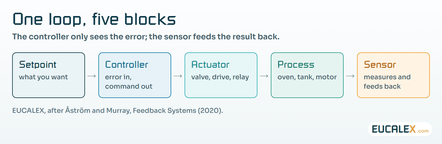
Two practical consequences follow. The loop can never be better than its sensor: a drifting probe gives you a perfectly controlled wrong value. And the loop can never be faster than its actuator allows. A valve that is fully open is no longer controlling anything, a point we come back to with windup.
What “good” means: precision, speed, stability
A loop is judged on a step, when the setpoint jumps or a disturbance hits, and three properties matter.
Precision is how close the output settles to the setpoint. The difference that remains is the static (or steady-state) error, usually expressed as a percentage of the setpoint.
Speed is how quickly the output reaches its final value and stays there. The usual measure is the settling time, the time after which the output stays inside a band around its final value. Åström and Murray use 2 %; many teaching texts use 5 %. Say which band you mean, or two engineers will argue about the same trace.
Stability means that, for a constant setpoint, the output converges. A loop that settles after a few decaying oscillations is stable but overshoots; one that keeps oscillating, or whose swings grow, is not acceptable.
The three pull against each other. More gain usually means less error and a faster response, right up to the point where it means overshoot, then oscillation. Tuning is choosing where to stand on that line for a given process.
Two kinds of process, and why they decide everything
The most useful question to ask before choosing a controller is this: if the command stays constant, does the process settle by itself?
Self-regulating processes do. An oven fed with constant power ends at the temperature where losses balance the heating. A pump running at constant speed into a tank with an open outlet ends at the level where outflow balances inflow. A motor at constant drive voltage ends at a constant speed.
Integrating processes do not. A motor that moves a carriage keeps moving as long as it is driven, because position is the integral of speed. A tank with no outlet keeps filling as long as the pump runs.
The difference matters because of what proportional control can and cannot do, and the four teaching rigs found in most automation courses show it clearly.
| Rig | Kind of process | Typical measurement | Proportional control alone |
|---|---|---|---|
| Mini oven with a solid-state relay | Self-regulating, slow, with a dead time | Pt100 probe, read by the PLC in tenths of a degree | A lasting error: heat is still needed to hold the temperature |
| Level column with an outlet valve | Self-regulating: the outlet sets the balance | 4–20 mA pressure transmitter | A lasting error: the pump must keep running |
| Motor speed through a variable-speed drive | Self-regulating, fast | Tachogenerator voltage | A lasting error that shrinks as the gain rises |
| Carriage position driven by a motor | Integrating: a stopped motor holds the position | Position encoder or ruler | No static error: a zero command holds the target |
The reason is simple. A proportional controller only produces a command when there is an error. If the process needs a non-zero command to stay at the setpoint (heat to cover losses, flow to cover the outlet), some error has to remain to produce it. An integrating process needs no command to stay where it is, so its error can go to zero. The oven also has a dead time: for a while after the heating changes, the probe sees nothing, and that delay is what makes aggressive tuning oscillate.
The four types of controller
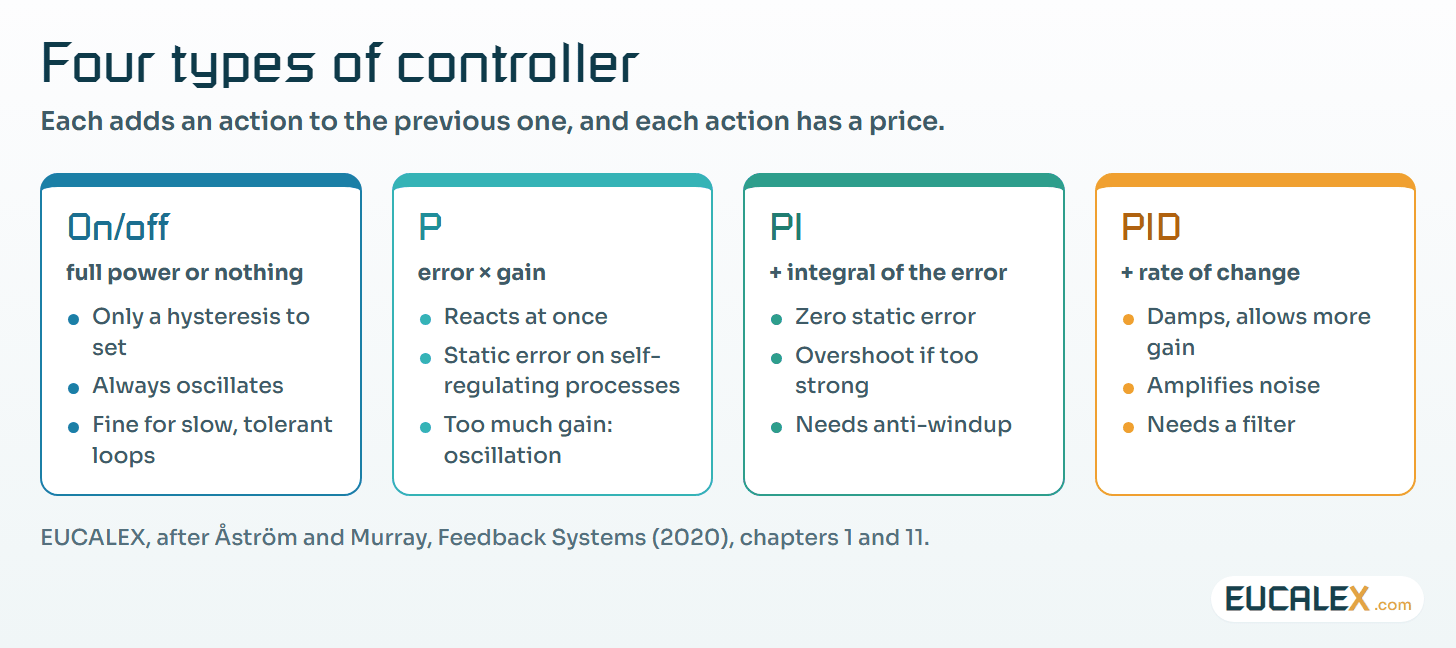
- On/off. Full power below the setpoint, nothing above it, usually with a small hysteresis so the relay does not chatter. Apart from the hysteresis there is nothing to tune, and on slow processes with a tolerance of a few degrees, a thermostat or a cold room, it is the right answer. It always oscillates around the setpoint, and the swing grows with the dead time.
- Proportional (P). The command is the error multiplied by a gain, limited to the actuator range. The band of error over which the output is not saturated is the proportional band. P removes most of the oscillation of on/off control, but on a self-regulating process it leaves the static error described above. Raising the gain shrinks that error until the loop starts to oscillate.
- Proportional-integral (PI). An integral term accumulates the error over time, so the command keeps growing as long as any error remains. If the loop reaches a steady state, the error is zero, a property Åström and Murray note is sometimes called the magic of integral action. The price is overshoot and slower settling when the integral is too strong. PI is what most temperature, level, flow and pressure loops on a plant actually run.
- Proportional-integral-derivative (PID). A derivative term reacts to the rate of change of the error and damps the response, which allows more gain and a faster loop. It also amplifies measurement noise, since noise is the fastest-changing thing in the signal, so industrial derivative terms are filtered. On noisy or slow loops the derivative is usually left at zero.
| Action | What it improves | What it costs |
|---|---|---|
| P | Reacts at once to any error; less static error as gain rises | Oscillation if the gain is too high; a lasting error on self-regulating processes |
| I | Removes the static error | Overshoot, slower settling, windup when the actuator saturates |
| D | Damps the response, allows a faster loop | Amplifies measurement noise; needs a filter |
What changes when a PLC runs the loop
Textbooks draw continuous signals. A PLC samples, scales, computes and clips, and each of those steps leaves its mark on the loop.
Scaling. Analogue signals arrive as integers. On a Siemens S7-1200, a 0–10 V input covers 0 to 27 648 in its rated range; values from 27 649 to 32 511 are already overrange (up to 11.759 V). A Pt100 input returns tenths of a degree, so 1 234 means 123.4 °C. A wrong scaling factor is an error you have calibrated in, and it survives every tuning session.
The sensor range catches people out too. A 4–20 mA transmitter reading 0–0.25 bar spans 0 to 2.549 m of water column (1 cm of water is 98.0665 Pa), not 2.5 m. Scale it as 0–250 cm and a full column reads about 2 % low. Small, but it is exactly the kind of error that turns up in a calibration report years later.
Sampling. The controller computes once per cycle or per cyclic interrupt. The period must be short compared with the dynamics of the process, stable, and known: an integral or derivative term computed with the wrong period is simply a different controller. Run control code in a cyclic interrupt with a fixed period, not in the free cycle whose duration wanders.
Saturation and windup. The command has to be limited to what the actuator accepts, 0 to 100 % of a valve or 0 to 10 V of a drive input. While it is saturated the loop is effectively open, and an integral term goes on accumulating error. When the error finally changes sign, the controller stays saturated for a long time and the process overshoots. That is integrator windup, and every serious implementation has anti-windup: Siemens documents the PID_Compact block supplied with the S7-1200 as a PIDT1 controller with anti-windup.
Noise and filtering. The derivative acts on the fastest part of the signal, which is usually noise. Filter the measurement or the derivative, and make sure the filter is slower than the noise but faster than the process.
On a regulated site, tuning is configuration
Gains, integral and derivative times, output limits, filters and setpoint ramps decide how a validated process behaves. Changing them is a change to the computerised system, and EU GMP Annex 11 makes no distinction between code and parameters:
“Any changes to a computerised system including system configurations should only be made in a controlled manner in accordance with a defined procedure.” EU GMP Annex 11, §10
In practice, record the tuning parameters of every GMP-relevant loop in the configuration baseline. Change them under change control, with a before-and-after step test. And put in the operational qualification a setpoint step and a disturbance for each critical loop, with acceptance criteria on error, settling time and overshoot. Our notes on change control and requalification and on degraded-mode OQ tests show how to size those tests, and recording a running PLC covers how to capture the trace without touching the controller.
Where to start
Eight steps are enough to bring a site’s loops under control:
- List the critical loops: controlled variable, sensor, actuator, where the controller runs, GMP impact.
- Classify each process as self-regulating or integrating, with or without dead time.
- Record the controller type and parameters as they are today, before anyone touches them.
- Check the scaling end to end: sensor range, transmitter signal, PLC integer, engineering units.
- Check the sampling: a fixed period, known, short compared with the process.
- Check the output limits and the anti-windup against the real actuator range.
- Step-test each critical loop and keep the trace: error, settling time, overshoot.
- Put the parameters under change control, with the step test as the acceptance evidence.
Five common mistakes
- Raising the gain to remove a static error on a self-regulating process. The error shrinks and the oscillation arrives. That error was a job for the integral term.
- Integral action without anti-windup. The loop behaves in normal operation and overshoots badly after every start-up or saturation.
- Derivative on a noisy measurement. The valve chatters and wears, and the loop ends up worse than it was with PI.
- Tuning on the wrong period. The controller is copied from one task to another, the cycle changes, and the same parameters now describe a different controller.
- Trusting the number without the scaling. A loop holding 100.0 cm on a sensor scaled 2 % wrong holds the wrong level, precisely and reproducibly.
Know what kind of process you drive before you touch a gain. Then write the gain down, because it is part of the validated system.
References
- Karl J. Åström and Richard M. Murray, *Feedback Systems: An Introduction for Scientists and Engineers*, 2nd edition, Princeton University Press, 2020.
- Siemens, *S7-1200 Programmable controller, System Manual*, A5E02486680-06: analogue value representation, RTD resolution, PID_Compact.
- NIST, Special Publication 811, Appendix B.9: conversion factors for the bar and the conventional centimetre of water.
- European Commission, EU GMP Annex 11: Computerised Systems, §10.
Related articles
All articles- Recording what a running PLC does: signal analysers, what they see, and what they change on a validated lineA PC-based signal analyser can show the fault nobody sees on the HMI. It can also write into the controller, open a remote path into the cell and…
- When the power and the air go away: designing the degraded-mode tests of an OQOperational qualifications test the normal path well and the failure path badly. What to observe when electrical power and compressed air are lost…
- When does a repair become a requalification? Change control on qualified equipmentA qualification report describes a machine on the day it was signed. Every repair, spare part and program edit after that day either keeps the…
EUCALEX
Have a project or a technical challenge?
Contact us: we will be pleased to discuss it with you, with no commitment.
Discuss your project with usStay informed
Receive new EUCALEX articles and technical insights by email.